Ben biraz keyfi olay dönemini seçmiş olsanız bile, oldukça doğru bir rakam çoğalır Verileri ve her bineyi bir etkinlik olarak ele almak. Ancak, şimdi ne olur, her olayda her olayda farklı sayıda işlem gerçekleştiğinden, her olay biraz farklıdır. Bu, aynı zamanda, bu sorunun üstesinden gelmek için önerilen bir yol ile bir Hawkes işlem bölümüne takılması Bitcoin Ticari Varış içinde the article ifade edilir: The only difference to the original dataset is that I added a random millisecond timestamp to all trades that share a timestamp with another trade. This is required as the model requires to distinguish every trade (i.e. every trade must have a unique timestamp). Bu, aşağıdaki kodu dahil edilmektedir:
import numpy as np
import math, matplotlib, pandas
import scipy.optimize
import matplotlib.pyplot
import matplotlib.lines
" Read example trades' data. "
all_trades = pandas.read_csv('all_trades.csv', parse_dates=[0], index_col=0) # All trades' data.
all_counts = pandas.DataFrame({'counts': np.ones(len(all_trades))}, index=all_trades.index) # Only the count of the trades is really important.
empirical_1min = all_counts.resample('1min', how='sum') # Bin the data so find the number of trades in 1 minute intervals.
baseEventTimes = np.array(range(len(empirical_1min.values)), dtype=np.float64) # Dummy times when the events take place, don't care too much about actual epochs where the bins are placed - this could be scaled to days since epoch, second since epoch and any other measure of time.
eventTimes = [] # With the event batches split into separate events.
for i in range(len(empirical_1min.values)): # Deal with many events occurring at the same time - need to distinguish between them by splitting each batch of events into distinct events taking place at almost the same time.
if not np.isnan(empirical_1min.values[i]):
for j in range(empirical_1min.values[i]):
eventTimes.append(baseEventTimes[i]+0.000001*(j+1)) # For every event that occurrs at this epoch enter a dummy event very close to it in time that will increase the conditional intensity.
eventTimes = np.array(eventTimes, dtype=np.float64) # Change to array for ease of operations.
" Find a fit for alpha, beta, and mu that minimises loglikelihood for the input data. "
#res = scipy.optimize.minimize(loglikelihood, (0.01, 0.1,0.1), method='Nelder-Mead', args = (eventTimes,))
#(mu, alpha, beta) = res.x
mu = 0.07 # Parameter values as found in the article.
alpha = 1.18
beta = 1.79
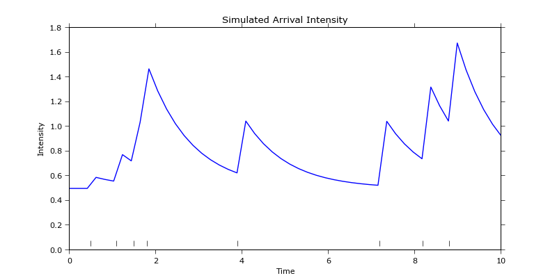
" Compute conditional intensities for all epochs using the Hawkes process - add more points to see how the effect of individual events decays over time. "
conditionalIntensitiesPlotting = [] # Conditional intensity for every epoch of interest.
timesOfInterest = np.linspace(eventTimes.min(), eventTimes.max(), eventTimes.size*10) # Times where the intensity will be sampled. Sample at much higher frequency than the events occur at.
for t in timesOfInterest:
conditionalIntensitiesPlotting.append(mu + np.array([alpha*math.exp(-beta*(t-ti)) if t > ti else 0.0 for ti in eventTimes]).sum()) # Find the contributions of all preceding events to the overall chance of another one occurring. All events that occur after time of interest t have no contribution.
" Compute conditional intensities at the same epochs as the empirical data are known. "
conditionalIntensities=[] # This will be used in the QQ plot later, has to have the same size as the empirical data.
for t in np.linspace(eventTimes.min(), eventTimes.max(), eventTimes.size):
conditionalIntensities.append(mu + np.array([alpha*math.exp(-beta*(t-ti)) if t > ti else 0.0 for ti in eventTimes]).sum()) # Use eventTimes here as well to feel the influence of all the events that happen at the same time.
" Plot the empirical and fitted datasets. "
fig = matplotlib.pyplot.figure()
ax = fig.gca()
labelsFontSize = 16
ticksFontSize = 14
fig.suptitle(r"$Conditional\ intensity\ VS\ time$", fontsize=20)
ax.grid(True)
ax.set_xlabel(r'$Time$',fontsize=labelsFontSize)
ax.set_ylabel(r'$\lambda$',fontsize=labelsFontSize)
matplotlib.rc('xtick', labelsize=ticksFontSize)
matplotlib.rc('ytick', labelsize=ticksFontSize)
# Plot the empirical binned data.
ax.plot(baseEventTimes,empirical_1min.values, color='blue', linestyle='solid', marker=None, markerfacecolor='blue', markersize=12)
empiricalPlot = matplotlib.lines.Line2D([],[],color='blue', linestyle='solid', marker=None, markerfacecolor='blue', markersize=12)
# And the fit obtained using the Hawkes function.
ax.plot(timesOfInterest, conditionalIntensitiesPlotting, color='red', linestyle='solid', marker=None, markerfacecolor='blue', markersize=12)
fittedPlot = matplotlib.lines.Line2D([],[],color='red', linestyle='solid', marker=None, markerfacecolor='blue', markersize=12)
fig.legend([fittedPlot, empiricalPlot], [r'$Fitted\ data$', r'$Empirical\ data$'])
matplotlib.pyplot.show()
Bu, aşağıdaki uygun üretir Arsa:  Her şey iyi görünüyor, ama detaylara baktığınızda, artık işlemlerin sayısının bir vektörünü alarak ve takılan parçanın çıkarılmasıyla artıkların farklı uzunluklara sahip olduklarından hesaplanmayacağını göreceksiniz. :
  Bu bir Bununla birlikte, ampirik veriler için kaydedildiği zamandaki aynı yoğunluktaki yoğunluğu ayıklamak ve daha sonra tortuları hesaplamak.
""" GENERATE THE QQ PLOT. """
" Process the data and compute the quantiles. "
orderStatistics=[]; orderStatistics2=[];
for i in range(empirical_1min.values.size): # Make sure all the NANs are filtered out and both arrays have the same size.
    if not np.isnan(empirical_1min.values[i]):
     orderStatistics.append(empirical_1min.values[i])
     orderStatistics2.append(conditionalIntensities[i])
orderStatistics = np.array(orderStatistics); orderStatistics2 = np.array(orderStatistics2);

orderStatistics.sort(axis=0) # Need to sort data in ascending order to make a QQ plot. orderStatistics is a column vector.
orderStatistics2.sort()

smapleQuantiles=np.zeros(orderStatistics.size) # Quantiles of the empirical data.
smapleQuantiles2=np.zeros(orderStatistics2.size) # Quantiles of the data fitted using the Hawkes process.
for i in range(orderStatistics.size):
    temp = int(100*(i-0.5)/float(smapleQuantiles.size)) # (i-0.5)/float(smapleQuantiles.size) th quantile. COnvert to % as expected by the numpy function.
    if temp<0.0:
     temp=0.0 # Avoid having -ve percentiles.
    smapleQuantiles[i] = np.percentile(orderStatistics, temp)
    smapleQuantiles2[i] = np.percentile(orderStatistics2, temp)

" Make the quantile plot of empirical data first. "
fig2 = matplotlib.pyplot.figure()
ax2 = fig2.gca(aspect="equal")

fig2.suptitle(r"$Quantile\ plot$", fontsize=20)
ax2.grid(True)
ax2.set_xlabel(r'$Sample\ fraction\ (\%)$',fontsize=labelsFontSize)
ax2.set_ylabel(r'$Observations$',fontsize=labelsFontSize)
matplotlib.rc('xtick', labelsize=ticksFontSize)
matplotlib.rc('ytick', labelsize=ticksFontSize)

distScatter = ax2.scatter(smapleQuantiles, orderStatistics, c='blue', marker='o') # If these are close to the straight line with slope line these points come from a normal distribution.

ax2.plot(smapleQuantiles, smapleQuantiles, color='red', linestyle='solid', marker=None, markerfacecolor='red', markersize=12)
normalDistPlot = matplotlib.lines.Line2D([],[],color='red', linestyle='solid', marker=None, markerfacecolor='red', markersize=12)

fig2.legend([normalDistPlot, distScatter], [r'$Normal\ distribution$', r'$Empirical\ data$'])
matplotlib.pyplot.show()

" Make a QQ plot. "
fig3 = matplotlib.pyplot.figure()
ax3 = fig3.gca(aspect="equal")

fig3.suptitle(r"$Quantile\ -\ Quantile\ plot$", fontsize=20)
ax3.grid(True)
ax3.set_xlabel(r'$Empirical\ data$',fontsize=labelsFontSize)
ax3.set_ylabel(r'$Data\ fitted\ with\ Hawkes\ distribution$',fontsize=labelsFontSize)
matplotlib.rc('xtick', labelsize=ticksFontSize)
matplotlib.rc('ytick', labelsize=ticksFontSize)

distributionScatter = ax3.scatter(smapleQuantiles, smapleQuantiles2, c='blue', marker='x') # If these are close to the straight line with slope line these points come from a normal distribution.

ax3.plot(smapleQuantiles, smapleQuantiles, color='red', linestyle='solid', marker=None,  markerfacecolor='red', markersize=12)
normalDistPlot2 = matplotlib.lines.Line2D([],[],color='red', linestyle='solid', marker=None, markerfacecolor='red', markersize=12)

fig3.legend([normalDistPlot2, distributionScatter], [r'$Normal\ distribution$', r'$Comparison\ of\ datasets$'])
matplotlib.pyplot.show()
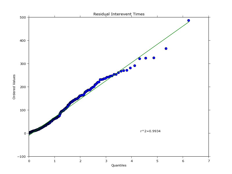
Bu, aşağıdaki araziler oluşturur: Bu, hem deneysel ve donatılmış veri miktarlarını bulmak ve böylece QQ arsa üreten birbirlerine karşı çizmek sağlar 

ampirik miktarsal arsa Veriler tam olarak the same as in the article değil, neden istatistiklerle harika olmadığımı bilmiyorum. Ancak, programlama açısından, bütün bunlar için nasıl gidebiliriz.

Bunun bir programlama sorusu olduğundan emin misiniz?En azından, herkese, atıfta bulunduğunuz kodun belgelerini okumaya zorlamadan, tam olarak ne yapmaya çalıştığınızı söyleyebilir misiniz? Bir bilim insanı olarak, eğer ihtiyacınız varsa, bazı yardım için yazarlarla temasa geçmenizi tavsiye ederim. Ancak onların kodlarını sizin için Python'a çevireceklerinden şüpheniz var. –
@AleksanderLidtke Hawkes modelinin ve Poisson modelinin sahip olduğum verilere ne kadar uyduğunu karşılaştırmak istiyorum. Bunu yapmanın iyi bir yolu varmış gibi görünüyorlardı, ama hepsi R'de. Python'daki verilerimde yeniden üretmek istiyorum. EvalCIF kodu, bir şekilde takılı modelle ampirik yoğunlukları (yani veriler) karşılaştırmak gibi görünüyor. – eleanora
Iletisim modellerinin QQ grafiklerini yaptigini biliyorum ama bu, kalıntılari ne yazık ki yaratmaya yardim etmiyor. – felix