Bu bir hız meselesidir. Üç davranış durumu vardır bir difüzyon denklemi çözmeye çalışıyorum burada:4. Sıra Runga Kutta Metodu - Difüzyon denklemi - Görüntü analizi
- Lambda == 0 denge
- Lambda> 0 max difüzyon
- Lambda < 0 dak difüzyon
Darboğaz, difüzyon operatör işlevindeki diğer ifadedir.
Denge durumu basit bir T işlemine sahiptir. ve ve Difüzyon operatörü. Diğer iki devlet için oldukça karmaşık hale geliyor. Ve şimdiye kadar kod çalıştırma süreleri boyunca oturup sabrım yoktu. Bildiğim kadarıyla denklemler doğru ve denge durumunun çıktısı doğru görünüyor, belki de birinin dengesiz durumların hızını arttırmak için bazı ipuçları var mı?
(yerine Runge-Kutta Euler çözeltisi (FTCS) daha çabuk hayal olurdu. Henüz bu denemedim.)
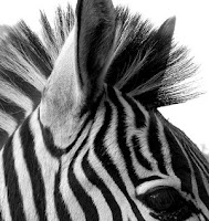
Dışarı kod denemek için herhangi bir siyah ve beyaz görüntü alabilirsiniz. Minimum ve maksimum olgu pahalı ve yavaş iken Kısaca
import numpy as np
import sympy as sp
import scipy.ndimage.filters as flt
from PIL import Image

# import image
im = Image.open("/home/will/Downloads/zebra.png")
arr = np.array(im)
arr=arr/253.

def T(lamda,x):
    """
    T Operator
    lambda is a "steering" constant between 3 behavior states
    -----------------------------
    0  -> linearity
    +inf -> max
    -inf -> min
    -----------------------------
    """
    if lamda == 0: # linearity
     return x
    elif lamda > 0: # Half-wave rectification
     return np.max(x,0)
    elif lamda < 0: # Inverse half-wave rectification
     return np.min(x,0)


def Diffusion_operator(lamda,f,t):
    """
    2D Spatially Discrete Non-Linear Diffusion
    ------------------------------------------
    Special case where lambda == 0, operator becomes Laplacian


    Parameters
    ----------
    D : int      diffusion coefficient
    h : int      step size
    t0 : int      stimulus injection point
    stimulus : array-like  luminance distribution

    Returns
    ----------
    f : array-like    output of diffusion equation
    -----------------------------
    0  -> linearity (T[0])
    +inf -> positive K(lamda)
    -inf -> negative K(lamda)
    -----------------------------
    """
    if lamda == 0: # linearity
     return flt.laplace(f)
    else:   # non-linearity
     f_new = np.zeros(f.shape)
     for x in np.arange(0,f.shape[0]-1):
      for y in np.arange(0,f.shape[1]-1):
       f_new[x,y]=T(lamda,f[x+1,y]-f[x,y]) + T(lamda,f[x-1,y]-f[x,y]) + T(lamda,f[x,y+1]-f[x,y])
       + T(lamda,f[x,y-1]-f[x,y])
     return f_new


def Dirac_delta_test(tester):
    # Limit injection to unitary multiplication, not infinite
    if np.sum(sp.DiracDelta(tester)) == 0:
     return 0
    else:
     return 1

def Runge_Kutta(stimulus,lamda,t0,h,N,D,t_N):
    """
    4th order Runge-Kutta solution to:
    linear and spatially discrete diffusion equation (ignoring leakage currents)

    Adiabatic boundary conditions prevent flux exchange over domain boundaries
    Parameters
    ---------------
    stimulus : array_like input stimuli [t,x,y]
    lamda : int    0 +/- inf
    t0 : int    point of stimulus "injection"
    h : int     step size
    N : int     array size (stimulus.shape[1])
    D : int     diffusion coefficient [constant]

    Returns
    ----------------
    f : array_like   computed diffused array

    """
    f = np.zeros((t_N+1,N,N)) #[time, equal shape space dimension]
    t = np.zeros(t_N+1)

    if lamda ==0:
     """ Linearity """
     for n in np.arange(0,t_N):
      k1 = D*flt.laplace(f[t[n],:,:]) +  stimulus*Dirac_delta_test(t[n]-t0)
      k1 = k1.astype(np.float64)
      k2 = D*flt.laplace(f[t[n],:,:]+(0.5*h*k1)) +  stimulus*Dirac_delta_test((t[n]+(0.5*h))- t0)
      k2 = k2.astype(np.float64)
      k3 = D*flt.laplace(f[t[n],:,:]+(0.5*h*k2)) + stimulus*Dirac_delta_test((t[n]+(0.5*h))-t0)
      k3 = k3.astype(np.float64)
      k4 = D*flt.laplace(f[t[n],:,:]+(h*k3)) + stimulus*Dirac_delta_test((t[n]+h)-t0)
      k4 = k4.astype(np.float64)
      f[n+1,:,:] = f[n,:,:] + (h/6.) * (k1 + 2.*k2 + 2.*k3 + k4)
      t[n+1] = t[n] + h
     return f

    else:
     """ Non-Linearity THIS IS SLOW """
     for n in np.arange(0,t_N):
      k1 = D*Diffusion_operator(lamda,f[t[n],:,:],t[n]) + stimulus*Dirac_delta_test(t[n]-t0)
      k1 = k1.astype(np.float64)
      k2 = D*Diffusion_operator(lamda,(f[t[n],:,:]+(0.5*h*k1)),t[n]) + stimulus*Dirac_delta_test((t[n]+(0.5*h))- t0)
      k2 = k2.astype(np.float64)
      k3 = D*Diffusion_operator(lamda,(f[t[n],:,:]+(0.5*h*k2)),t[n]) + stimulus*Dirac_delta_test((t[n]+(0.5*h))-t0)
      k3 = k3.astype(np.float64)
      k4 = D*Diffusion_operator(lamda,(f[t[n],:,:]+(h*k3)),t[n]) + stimulus*Dirac_delta_test((t[n]+h)-t0)
      k4 = k4.astype(np.float64)
      f[n+1,:,:] = f[n,:,:] + (h/6.) * (k1 + 2.*k2 + 2.*k3 + k4)
      t[n+1] = t[n] + h

     return f

# Code to run
N=arr.shape[1] # Image size
stimulus=arr[0:N,0:N,1]
D = 0.3 # Diffusion coefficient [0>D>1]
h = 1  # Runge-Kutta step size [h > 0]
t0 = 0 # Injection time
t_N = 100 # End time

f_out_equil = Runge_Kutta(stimulus,0,t0,h,N,D,t_N)
f_out_min = Runge_Kutta(stimulus,-1,t0,h,N,D,t_N)
f_out_max = Runge_Kutta(stimulus,1,t0,h,N,D,t_N)
, f_out_equil hesaplamak için nispeten hızlıdır. Benim kodlama takdir çok teşekkür ederiz iyileştirmeye http://4.bp.blogspot.com/_KbtOtXslVZE/SweZiZWllzI/AAAAAAAAAIg/i9wc-yfdW78/s200/Zebra_Black_and_White_by_Jenvanw.jpg
İpuçları, İşte
çıkışıimport matplotlib.pyplot as plt
fig1, (ax1,ax2,ax3,ax4,ax5) = plt.subplots(ncols=5, figsize=(15,5))
ax1.imshow(f_out_equil[1,:,:],cmap='gray')
ax2.imshow(f_out_equil[t_N/10,:,:],cmap='gray')
ax3.imshow(f_out_equil[t_N/2,:,:],cmap='gray')
ax4.imshow(f_out_equil[t_N/1.5,:,:],cmap='gray')
ax5.imshow(f_out_equil[t_N,:,:],cmap='gray')
Kodunuzun doğru çalıştığından emin misiniz? Son birkaç satırda parantez hataları var – Alessandro
şimdi iyi olmalı – WBM
Ben google bulundu ilk zebra b/w görüntü ile şekil hatası olsun, belki sizin örnek için çalışan bir dosya bağlantısı sağlayabilir. Burada – Alessandro